Prior to the era of reproducible research, it was quite common for published graphs, charts, and other figures to be released solely as static images such and PNGs or JPEGs. Often times this is not done with accompanying code, or with the plot data available as a separate download, making it difficult to either reproduce or validate the findings.
We’ve talked about the virtues of the magick package in the past, and it turns out magick provides us with a way of extracting data from images. The exact details vary depending on the properties of the plot, including its saturation, lightness, and hue, but some general themes emerge. We wanted to briefly document one particular instance of this problem.
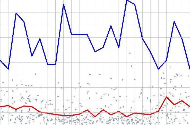
Consider the following image:

How can we reproduce this chart by extracting the data points and ultimately plotting in ggplot2? First, we read the image in with Magick:
library(tidyverse)
library(magick)

im <- image_read("line.jpg")
The first thing we will do is extract the saturation channel. Depending on the image, we may want to choose a different channel here - in this case, however, the lines are the most saturated part of the image, and therefore the saturation is the most distinguishable characteristic of the chart. When we extract the saturation, we use the following code and obtain the following image:
im_proc <- im %>%
    image_channel("saturation")

im_proc

You'll see that we now have a grayscale image, where darker values represent areas of lower saturation, in this case the points, and in particular the lines we are interested in. Next, we will threshold this image at 30%, so that any pixel value that is over 30% saturation gets set to white - this will effectively eliminate all pixels aside from the lines.
im_proc2 <- im_proc %>%
    image_threshold("white", "30%")

im_proc2

Finally, we will negate the image so that the lines are white and the rest are black. This ensures that any pixel value in the image higher than 0 (as white is) represents a point which we will choose to extract.
im_proc3 <- im_proc2 %>%
    image_negate()

im_proc3

Our final step is to perform some data manipulation with the tidyverse in order to convert the pixel values to points suitable for plotting in ggplot2.
dat <- image_data(im_proc3)[1,,] %>%
    as.data.frame() %>%
    mutate(Row = 1:nrow(.)) %>%
    select(Row, everything()) %>%
    mutate_all(as.character) %>%
    gather(key = Column, value = value, 2:ncol(.)) %>%
    mutate(Column = as.numeric(gsub("V", "", Column)),
           Row = as.numeric(Row),
           value = ifelse(value == "00", NA, 1)) %>%
    filter(!is.na(value))
And then we plot:
ggplot(data = dat, aes(x = Row, y = Column, colour = (Column < 300))) +
    geom_point() +
    scale_y_continuous(trans = "reverse") +
    scale_colour_manual(values = c("red4", "blue4")) +
    theme(legend.position = "off")

And there you have it! We'd love any feedback or enhancements to this method, especially ones that may pertain to more general cases. We hope you enjoyed!